The problem
The cost of learning prototypes
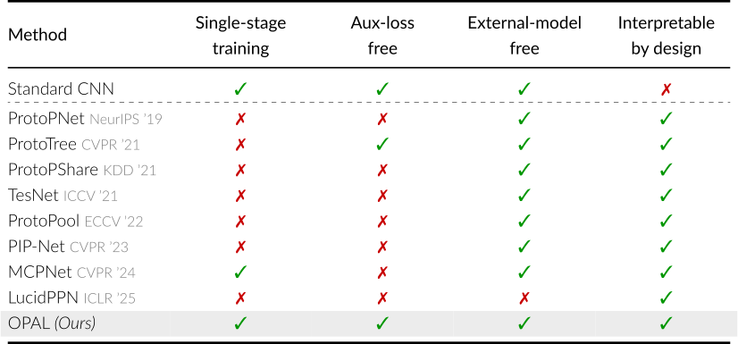
Part-prototype models are interpretable by design: a prediction is grounded in localized visual evidence. Learning those prototypes is what makes them expensive, because representation learning and prototype alignment have to converge jointly.
Abstract
Interpretability as representation alignment
Prototypical part-based models provide explainable predictions by comparing input regions to learned prototypes. However, current approaches are burdened by complex, multi-stage training pipelines and heavily rely on auxiliary regularization to prevent prototype collapse. To overcome these limitations, we introduce Orthonormal Prototype Alignment Learning (OPAL), a single-stage, end-to-end framework that simplifies interpretable classification. Our approach anchors the latent space using predefined orthonormal bases, embedding each class within a dedicated subspace spanned by fixed part-prototypes. To achieve precise part localization, OPAL enforces spatial competition across feature maps. This mechanism isolates sparse, discriminative regions, directing each prototype to consistently attend to the same semantic concept across different images. By framing classification as a direct representation alignment task, our method eliminates the need for auxiliary losses. Extensive experiments on fine-grained benchmarks demonstrate that OPAL outperforms both its non-interpretable counterparts and state-of-the-art part-prototype methods, delivering granular visual explanations by explicitly revealing the specific image regions driving every prediction.
Key idea
From prototype discovery to structured alignment
Prior work searches for prototypes in an unconstrained latent space, where evidence from different classes can overlap. OPAL preassigns the geometry instead: each class \(c\) spans its own orthonormal subspace \(\mathcal{S}_c \subset \mathbb{R}^{K}\), and the only thing left to learn is the representation that aligns to it.
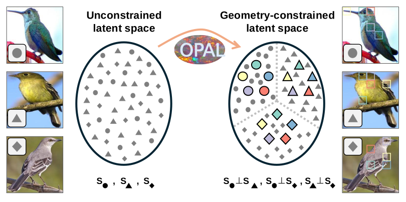
- Fix the directions, not the features. Part-prototypes are preassigned to canonical orthonormal axes and never updated, which removes the moving-target coupling between prototype optimization and representation learning.
- Orthogonality structures parts and classes at once. Each class spans \(m\) orthonormal prototype directions, and the class subspaces are mutually orthogonal, so separation is a property of the design rather than of a loss term.
- One objective is enough. Training is cross-entropy over distances to the fixed anchors: no warm-up, no projection step, no alternating optimization, no auxiliary regularizers.
Tap the table to open it full size.
Method
OPAL: Orthonormal Prototype Alignment Learning
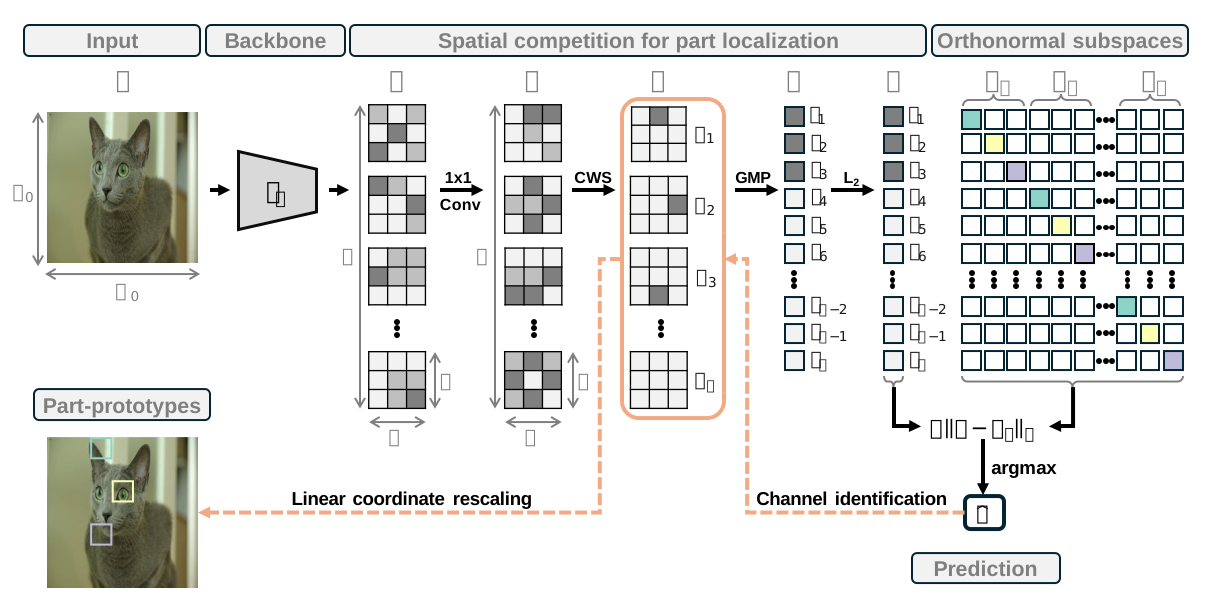
A backbone feature map is projected onto \(K = C \cdot m\) prototype coordinates. Channels compete for every spatial location, each surviving channel contributes exactly one image region, and the resulting embedding is classified by its distance to fixed orthonormal class anchors.
-
Project
A \(1\times1\) convolution maps the backbone feature map \(F \in \mathbb{R}^{D\times H\times W}\) to \(G \in \mathbb{R}^{K\times H\times W}\) with \(K = C\cdot m\), so every class \(c\) owns a block \(B_c\) of \(m\) prototype slots.
-
Compete
A channel-wise softmax normalizes across channels at each location, so \(\sum_{k} A_k(u,v) = 1\) everywhere and a single image region cannot support several prototypes at once.
\[ A_k(u,v) \;=\; \frac{\exp\!\big(G_k(u,v)\big)}{\sum_{j=1}^{K} \exp\!\big(G_j(u,v)\big)} \] -
Localize
Global max pooling keeps one response per channel together with its maximizer, and \(L_2\) normalization gives \(z = s / \lVert s \rVert_2\). Each coordinate of \(z\) is therefore sourced from exactly one spatial location, whose image patch is the evidence behind that coordinate.
\[ s_k \;=\; \max_{(u,v)\in\Omega} A_k(u,v), \qquad (u_k^{*}, v_k^{*}) \;=\; \arg\!\max_{(u,v)\in\Omega} A_k(u,v) \] -
Align
Each class is represented by a fixed block-uniform anchor \(a_c\), unit-norm and orthogonal to every other anchor. Logits are negative distances, and training is plain cross-entropy over them: since \(z\) and \(a_c\) are both unit-norm, this is equivalent to maximizing cosine similarity on the hypersphere.
\[ a_c \;=\; \frac{1}{\sqrt{m}}\sum_{j=1}^{m} p_{c,j}, \qquad \ell_c \;=\; -\lVert z - a_c \rVert_2 \] -
Explain by construction
For the predicted class \(\hat{y}\), the \(m\) channels of block \(B_{\hat{y}}\) each contribute one maximizer. Rescaling those coordinates from the \(H\times W\) grid back to the \(H_0\times W_0\) input resolution yields the part-prototype evidence, with no attribution method in between.
Quantitative results
Accuracy, generalization and efficiency
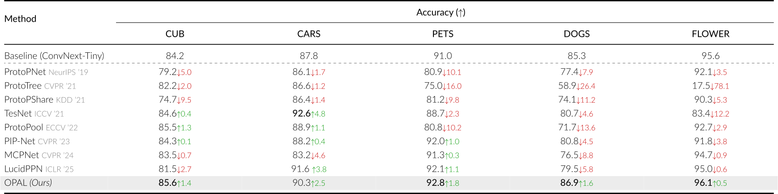
Top-1 accuracy on CUB-200-2011, Stanford Cars, Oxford-IIIT Pet, Stanford Dogs and Oxford Flowers-102. All numbers are means over three seeds under an identical protocol; arrows are absolute percentage-point differences with respect to the corresponding CNN backbone.
Comparison with inherently interpretable models
Tap the table to open it full size.
- Leading performance. OPAL ranks first on 4 of the 5 benchmarks and remains competitive on CARS, where it is third behind TesNet and LucidPPN.
- No accuracy trade-off. It is the only method that stays above its own ConvNeXt-Tiny backbone on all five datasets, by \(+1.56\) points on average, while every competitor loses accuracy on at least two of them.
Backbone generalization and scalability
Three convolutional families at three scales each — ResNet-50/101/152, EfficientNet-V2 S/M/L and ConvNeXt Tiny/Small/Base — are trained in their standard form and with the OPAL head under the same protocol, which isolates the contribution of the head from backbone-specific design choices.
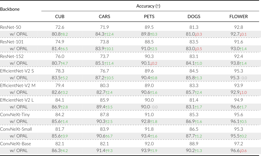
Tap the table to open it full size.
- Backbone-agnostic gains. OPAL improves or matches the non-interpretable counterpart in 39 of 45 backbone–dataset settings, by \(+2.94\) points on average.
- Robust in the failure cases. Where it does not improve, the largest single drop across all 45 settings is 1.0 point.
Computational overhead
The OPAL head replaces the linear classifier with a \(1\times1\) projection to \(K = C\cdot m\) channels, so its cost is dataset-dependent and grows with the number of classes. The question is whether that cost is material next to the feature extractor.
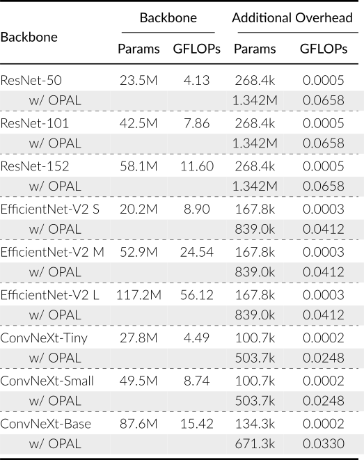
Tap the table to open it full size.
- Cheap to add. Averaged over backbones and datasets, the OPAL head accounts for 2.36% of the backbone parameters and 0.53% of its GFLOPs, so the feature extractor remains the dominant cost.
Qualitative analysis
What the model actually looks at
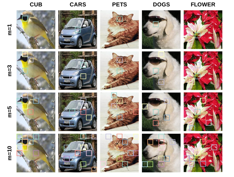
Every explanation below is read directly off the forward pass: for the predicted class, each of its \(m = 5\) prototype channels contributes the single image location that produced its pooled response. Nothing is recomputed and no attribution method is involved.
Prototype-based explanations
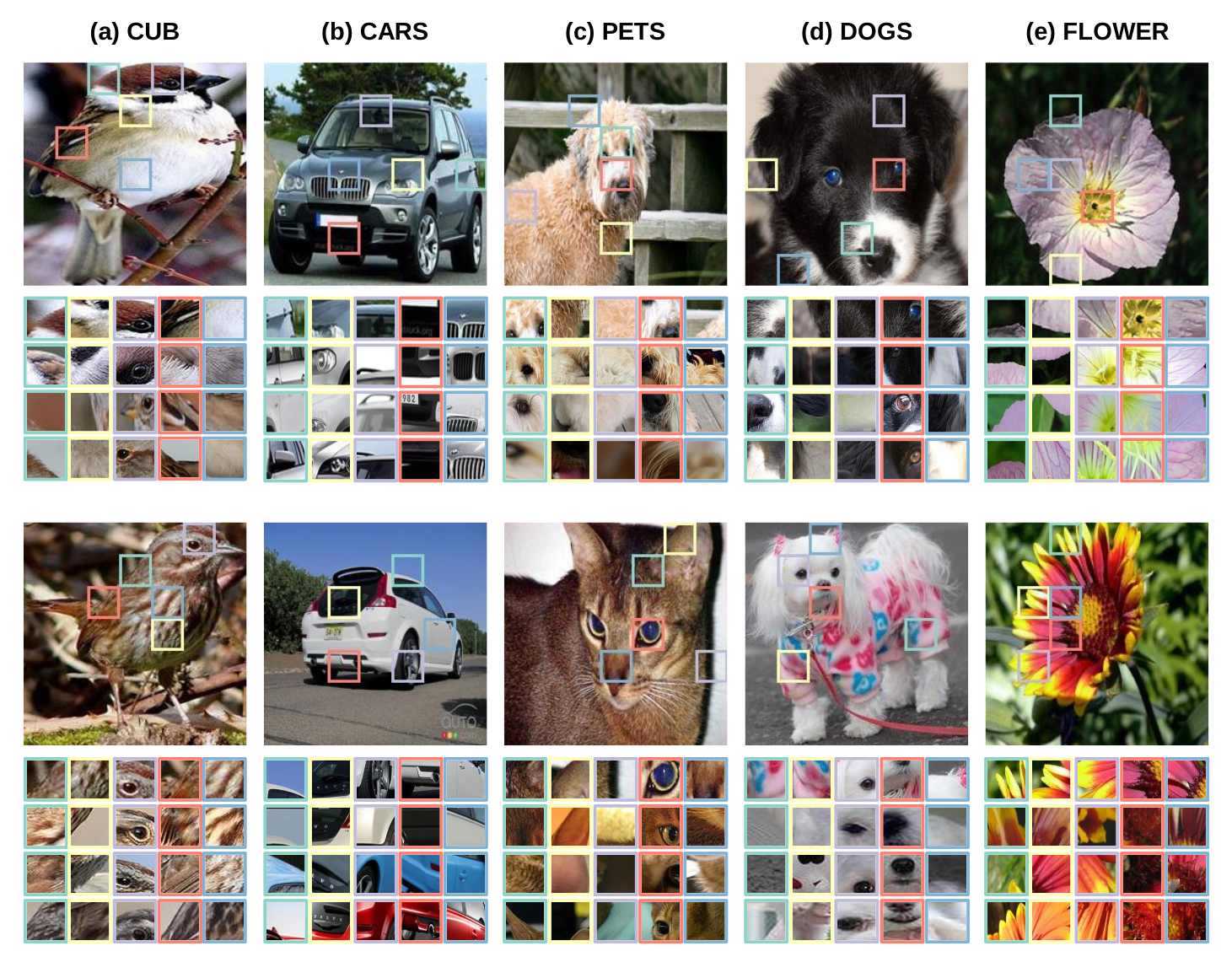
- Complementary evidence. The \(m\) slots spread over distinct discriminative parts of the object instead of concentrating on one salient region — which is what fine-grained recognition needs, since class separation often depends on subtle part-level attributes.
- Consistent semantics. The same slot repeatedly selects the same part across different images of a class: ears for Abyssinian cats in PETS, eyes for Maltese dogs in DOGS.
Understanding prototype diversity
Two design choices control what the explanations look like: the channel-wise softmax, which makes prototypes compete for spatial locations, and \(m\), which sets how many parts each class is allowed to use.
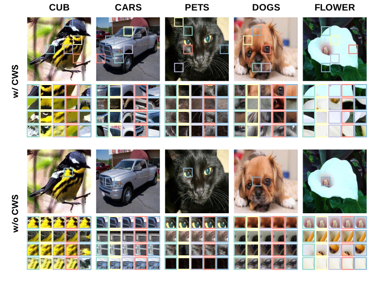
- Competition prevents collapse. Measured by the Spatial Prototype Collapse score, the variant without channel-wise softmax reaches 72.1–93.6 across datasets, while full OPAL stays at 4.9 or below.
- Granularity is controlled by \(m\). A single parameter trades representational capacity against discriminative focus, and its qualitative effect mirrors the accuracy trend measured below.
Quantifying prototype quality
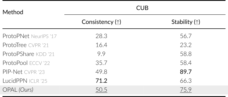
CUB-200-2011 is the only one of the five benchmarks with part-level annotations, so prototype consistency — whether a prototype keeps selecting the same annotated body part across images of its class — and stability — whether that association survives input noise — are reported there.
Tap the table to open it full size.
- High prototype quality. OPAL is second best on both metrics, at 50.5 consistency and 75.9 stability.
- Competitive without specialized machinery. The two per-metric leaders rely on it: LucidPPN on an external part-discovery model for initial prototype alignment, PIP-Net on a self-supervised prototype warm-up stage and auxiliary losses. OPAL needs neither.
Understanding design choices
What each component contributes
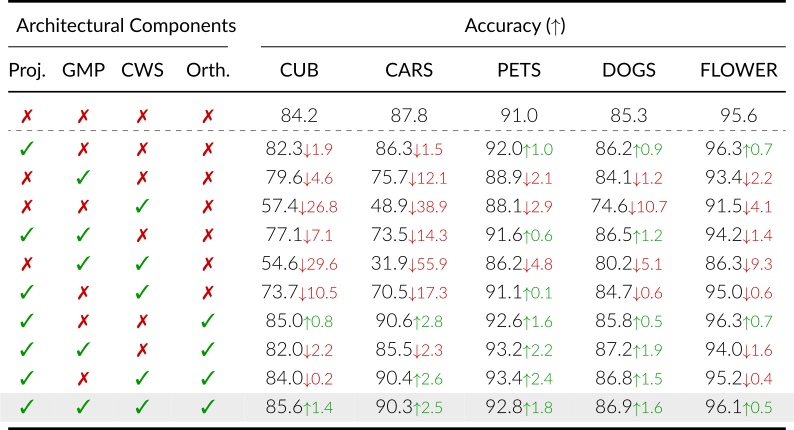
The \(1\times1\) projection (Proj.), global max pooling (GMP), channel-wise softmax (CWS) and orthonormal anchors (Orth.) are enabled one combination at a time. All crosses is the plain convolutional baseline; all checks is full OPAL.
Architectural ablation
Tap the table to open it full size.
- Geometry is the key ingredient. Enabling orthonormal anchoring improves the matched non-orthogonal variants by \(+4.07\) points on average.
- Localization alone is not enough. Configurations that pool with GMP but without Orth. fall 9.86 points below the baseline while still producing perfectly localized evidence.
- The components are complementary. Some ablated variants win on isolated datasets, but they forfeit what OPAL is built for: dropping GMP breaks the one-maximizer-per-channel correspondence, dropping CWS removes the competition that keeps prototypes distinct.
Sensitivity to the number of prototypes per class
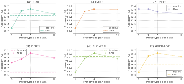
- One slot per class is insufficient. \(m = 1\) underperforms the baseline by 1.04 points on average.
- Moderate budgets work best. \(m \in \{3,5,10\}\) all sit above the baseline, by \(+1.25\) points on average; too many slots dilute the discriminative evidence, which makes \(m = 5\) the operating point used throughout.
Take-home message
Fix the prototype directions, learn the representation
- Orthonormal anchoring replaces the pipeline. Preassigning the class geometry makes single-stage, auxiliary-loss-free interpretable learning possible: one objective, one training run, image-level labels only.
- Interpretability without an accuracy penalty. OPAL yields diverse, localized evidence while improving or matching its non-interpretable counterpart in 39 of 45 backbone–dataset settings.
Take-away results
Resources
Paper, code, poster and video
Citation
If OPAL is useful in your work, please cite it
@inproceedings{carretero2026opal,
  title     = {OPAL: Orthonormal Prototype Alignment Learning for Interpretable Image Classification},
  author    = {Carretero, Il\'an and Angulo, Gustavo Jes\'us and del Amor, Roc\'io and Naranjo, Valery},
  booktitle = {European Conference on Computer Vision (ECCV)},
  year      = {2026}
}